

Having used Rob Hyndman’s forecasting package in R, I decided to give Facebook’s Prophet package a spin and do a comparison of the results.
##Forecasts using Prophet
The Time-series data sets: - Daily data set
##    y         ds
## 1  8 2016-05-10
## 2 10 2016-05-11
## 3  3 2016-05-11
## 4  7 2016-05-12
## 5  3 2016-05-12
## 6  3 2016-05-12
Prophet provides the ability to forecast projected growth based on market intel, by specifying the carrying capacity ‘cap’; the forecast should reach the maximum/saturation at the set ‘cap’. For this data set, I’ve set the cap at 7 units/day, but the forecaster can choose to set it at an increasing/decreasing sequence.
daily_Data_wgrowth <- daily_data %>%
  mutate(cap = 7)
head(daily_Data_wgrowth)
## y ds cap
## 1 8 2016-05-10 7
## 2 10 2016-05-11 7
## 3 3 2016-05-11 7
## 4 7 2016-05-12 7
## 5 3 2016-05-12 7
## 6 3 2016-05-12 7Visualize the daily timeseries
ggplotly(ggplot(daily_data, aes(x = ds, y = y)) + geom_line(color = "firebrick") + ggtitle("Daily Timeseries")) Functions calling function prophet that fits and returns the model, then predicts on the model object. More info available from Prophet’s page
#Function to apply prophet model to timeseries
prophet_apply <- function(timeseries, growthtype = NULL) {
  if(is.null(growthtype))
     prophet(timeseries)
    else
      prophet(timeseries, growth = growthtype)
}

#Create future data_frame and predict on the model object
prophet_fcst_apply <-
  function(m,
           length_time,
           cap_size = NULL) {
    if (is.null(cap_size))
    { future_df <- make_future_dataframe(m, periods = length_time)
    }
    else
    { future_df <- make_future_dataframe(m, periods = length_time)
      future_df['cap'] = cap_size
    }

  fcst_df <- predict(m, future_df)
  }
Model and forecast with prophet:
model_daily <- prophet_apply(daily_data)## Initial log joint probability = -46.2524
## Optimization terminated normally:
## Convergence detected: relative gradient magnitude is below tolerancemodel_daily_wgrowth <- prophet_apply(daily_Data_wgrowth, 'logistic')## Initial log joint probability = -13.2458
## Optimization terminated normally:
## Convergence detected: relative gradient magnitude is below toleranceFcst_daily <- prophet_fcst_apply(model_daily, 730)
Fcst_daily_wgrowth <- prophet_fcst_apply(model_daily_wgrowth, 730, 7)View forecasted units with their upper/lower confidence interval
#Select forecast with lower/upper confidence intervals from the predicted object
#Specify time frame for selection
view_select_Fcst <- function(fcst_df, date_begin, date_end) {
  selected_Fcst <- fcst_df %>%
    filter(ds >date_begin  & ds< date_end) %>%
    select(ds, yhat, yhat_lower, yhat_upper)
}

tail(view_select_Fcst(Fcst_daily, "2017-04-01", "2018-04-01"))
## ds yhat yhat_lower yhat_upper
## 360 2018-03-27 5.568770 1.2557720 9.688349
## 361 2018-03-28 5.449173 1.1129391 9.736892
## 362 2018-03-29 5.286332 0.9718378 9.680816
## 363 2018-03-30 5.475638 1.5285363 9.935465
## 364 2018-03-31 4.480532 0.3557986 8.664323
## 365 2018-04-01 5.195860 1.3188466 9.543473Visualize the forecast by calling the generic plot function. I’m wrapping ggplotly(via Plotly package) around the plot function for interactive web-based version.
Plots for forecasted daily data:
#Plot function for daily fcst
plot_daily <- function(m, fcst, fnc) {
    fnc(m, fcst)
}

ggplotly(plot_daily(model_daily, Fcst_daily, plot))
plot_daily(model_daily, Fcst_daily, prophet_plot_components)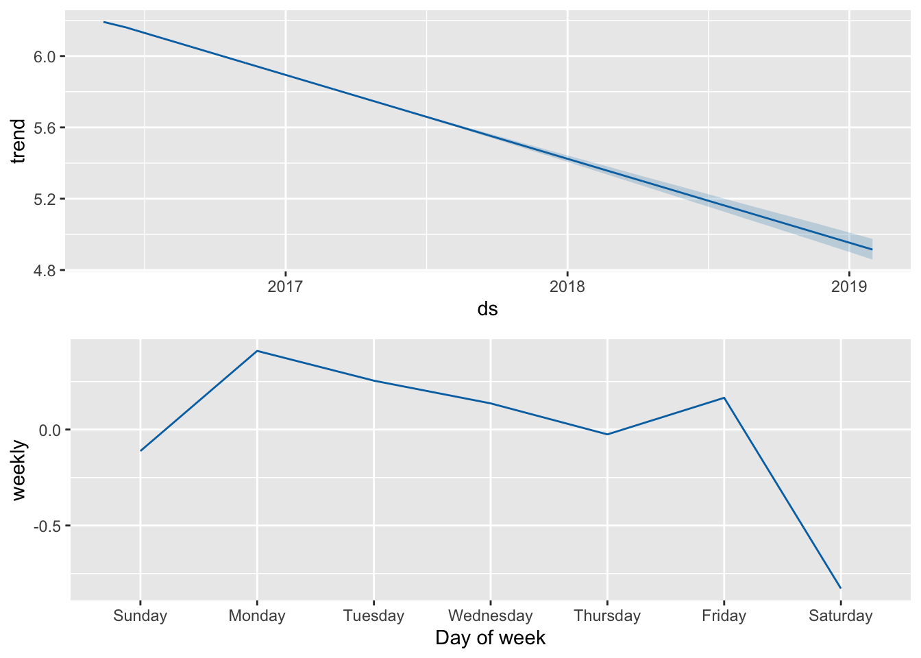
Sum forecast unit totals and forecast order dollars based on user specified price (in this case. price is set at $25).
#summarise yearly forecast units and order dollars
summary_fcst_units_price <- function(df, price, fcst_num) {
  df %>%
   dplyr::summarise(Fcst_qty = sum(df[[fcst_num]]), Fcst_Dlrs = Fcst_qty*price)
}
Daily data set:
#Call summary_fcst_units_price function on the predicted daily numbers
sum_daily <- summary_fcst_units_price(view_select_Fcst(Fcst_daily, "2017-04-01", "2018-04-01"), 25, "yhat")
sum_daily
## Fcst_qty Fcst_Dlrs
## 1 2022.837 50570.94Plots for daily_data with growth
ggplotly(plot_daily(model_daily_wgrowth, Fcst_daily_wgrowth, plot))plot_daily(model_daily_wgrowth, Fcst_daily_wgrowth, prophet_plot_components)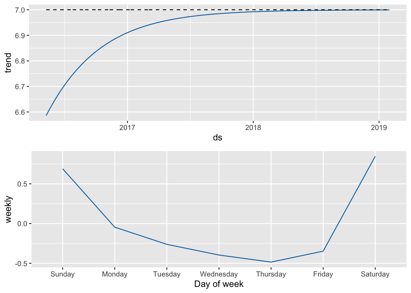
Daily_data with growth set:
tail(view_select_Fcst(Fcst_daily_wgrowth, "2017-04-01", "2018-04-01"))## ds yhat yhat_lower yhat_upper
## 360 2018-03-27 6.733838 2.182734 11.12016
## 361 2018-03-28 6.599399 2.431310 11.28659
## 362 2018-03-29 6.510695 2.053849 11.02729
## 363 2018-03-30 6.648348 1.935214 11.06018
## 364 2018-03-31 7.842190 3.437448 11.95472
## 365 2018-04-01 7.684945 3.518858 11.78566sum_daily_wgrowth <- summary_fcst_units_price(view_select_Fcst(Fcst_daily_wgrowth, "2017-04-01", "2018-04-01"),25, "yhat")
sum_daily_wgrowth## Fcst_qty Fcst_Dlrs
## 1 2548.958 63723.95Forecasts using Forecast Package by Hyndman
Using Auto ETS:
#Auto ETS forecast
daily_ts <- ts(daily_data[,1], start(2016,1,1), frequency = 7)
daily_auto_fcst <- forecast(daily_ts, h = 365)
#autoplot(daily_auto_fcst)
ggplotly(autoplot(daily_auto_fcst))
Sum total units and total order dollars based on price at $25
sum_hyndman_ets <- summary_fcst_units_price(data.frame(daily_auto_fcst), 25, "Point.Forecast")Using Auto Arima:
#Auto Arima Forecast
fit_ar_daily<- auto.arima(daily_ts)
daily_auto_ar_fcst <- forecast(fit_ar_daily, h = 365)
#autoplot(daily_auto_fcst)
ggplotly(autoplot(daily_auto_fcst))
sum_hyndman_ar <- summary_fcst_units_price(data.frame(daily_auto_ar_fcst), 25, "Point.Forecast")Let’s now compare the forecast results from Prophet and Forecast package by Hyndman
All_TS_fcst <- full_join(full_join(sum_daily, sum_daily_wgrowth), full_join(sum_hyndman_ets, sum_hyndman_ar))
rownames(All_TS_fcst) <- c("Fcst_daily_prophet", "Fcst_daily_wgrowth_prophet", "Fcst_daily_forecast_ETS", "Fcst_daily_forecast_ARIMA")
knitr::kable(All_TS_fcst, caption = "Forecasts from Prophet & Forecast Package")| Fcst_qty | Fcst_Dlrs | |
|---|---|---|
| Fcst_daily_prophet | 2022.837 | 50570.94 |
| Fcst_daily_wgrowth_prophet | 2548.958 | 63723.95 |
| Fcst_daily_forecast_ETS | 2251.012 | 56275.30 |
| Fcst_daily_forecast_ARIMA | 2250.967 | 56274.18 |
Share this post
Twitter
Google+
Facebook
Reddit
LinkedIn
StumbleUpon
Pinterest
Email